
Apache Arrow - The Missing Deep Dive Series - Part 2
How Apache Arrow Stores Data in Memory?

In my last post, I discussed why we need Apache Arrow—its reason for existence. In short, Arrow itself is not a tool. It's a specification standardizes how different programs store columnar data in memory to make them portable across processes, disk, and network.
Today, we will take a deep dive into how Apache Arrow stores a tabular data set in memory. After reading this post, you will learn:
Arrow represents data in a column-oriented format.
Columns of a tabular data set are represented using Arrow Arrays.
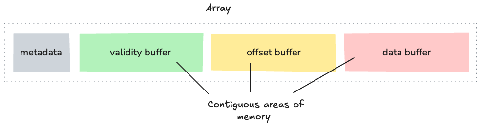
Each array is a self-contained unit of metadata and one or more buffers holding its data.
The physical memory representation describes how arrays are laid out in memory by Arrow, based on the type of data the arrays hold.
Arrow internal details are quite complicated. But we can always learn complex topics by relating them to something that we already know, breaking it down to smaller pieces, and trying to weave them together to derive knowledge. That is exactly what I’m going to do today.
So, let me take a simple tabular data set and see how Arrow will lay that out in memory for us, giving us a great way to start our discussion.
Arrow is columnar
We can represent a tabular data set in memory either in a row-oriented fashion or a column-oriented (columnar) format. The row-oriented format stores data row-by-row, meaning the rows are arranged adjacent to each other in computer memory:

Columnar format arranges data by columns instead of rows. Values for each column are laid out in contiguous blocks of memory.
For example, this is the same tabular data being saved in memory column by column.

Apache Arrow provides a standardized specification for columnar memory layout across programming languages. This means Arrow views our tabular data set simply as a collection of columns.
So, what are the benefits of storing tabular data in columnar format?
Memory Locality: Columnar organization makes analytical operations (filtering, grouping, aggregations) more efficient because related data is stored close together in memory. When the CPU processes this data, it accesses memory locations that are near each other.
Contiguous Memory: By storing column data in continuous memory blocks, Arrow enables better performance and more efficient use of the memory cache.
Vectorization and SIMD support: Columnar format enables vectorized computing, where operations can be performed on multiple data elements simultaneously using SIMD instructions (Single Instruction, Multiple Data). Most modern CPUs have these capabilities that can process multiple values at once with a single CPU instruction, significantly speeding up data processing operations. This is what we discussed a few weeks ago.
Columns as Arrow Arrays
Next, let's explore something interesting: how Arrow represents columns in memory.
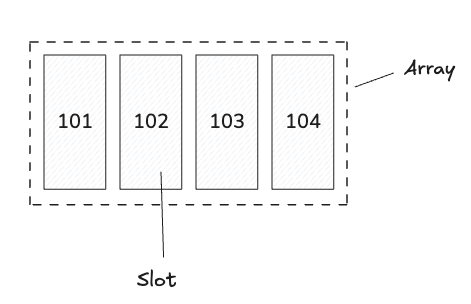
In Arrow terminology, each column of a tabular data set is represented as an Array. Arrow arrays are a sequence of values with known length, all having the same type. A Slot is what we call a single logical value in an array of some particular data type.
Later, you will see how related arrays can be grouped to derive the original tabular data set, allowing us to perform efficient computations on them.
Before we get there, let’s see how Arrow specification represents an array in memory. This is what we call a physical memory layout of an array, describing how the array’s data is laid out in memory.
Arrays are stored using Buffers
Values in an array are stored in one or more Buffers. A buffer is a sequential virtual address space (i.e., block of memory) with a given length. Given a pointer specifying the memory address where the buffer starts, you can reach any byte in the buffer with an “offset” value that specifies a location relative to the start of the buffer.
An array consists of one or more buffers. The number of buffers associated with an array depends on the exact type of data being stored.
For example, we can represent the Customer ID column in our data set as an array of signed 32 bit integers. When laid out in memory, an integer array consists of two pieces of metadata and two buffers that store the data. The metadata specify the length of the array and a count of the number of null values, both stored as 64-bit integers.
Before we find out what exactly goes into each buffer, it’s important to know about memory alignment of buffers.
Buffer memory alignment
Memory alignment refers to how data is arranged in memory relative to address boundaries. In Arrow, implementations are recommended to allocate memory on aligned addresses (multiple of 8- or 64-bytes) and pad to a length that is a multiple of 8 or 64 bytes.
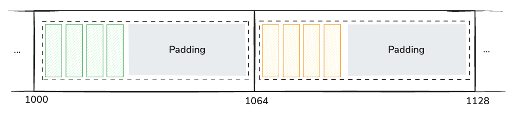
In most cases, Arrow uses 64-byte buffer lengths (or multiples of 64 bytes). This means the starting address of each buffer is a multiple of 64 bytes. Let’s say if a buffer starts at memory address 1000, the next buffer would start at address 1064, 1128, or another address divisible by 64, regardless of the actual data size.
For example, if a buffer contains 10 integers (40 bytes of data), it might actually be allocated with 64 bytes of memory, with the last 24 bytes being unused padding. This ensures that the next buffer starts at a 64-byte aligned address.
This memory alignment helps Arrow to achieve several benefits, especially optimized for CPU cache lines and SIMD operations.
Optimizes for CPU cache lines: Modern CPUs typically have 64-byte cache lines, so aligning data to these boundaries minimizes cache misses.
Enhances SIMD performance: SIMD instructions operate on multiple data elements simultaneously. Properly aligned memory ensures optimal SIMD performance since most SIMD instructions require aligned memory access.
Reduces padding overhead: By standardizing on 64-byte multiples, Arrow minimizes wasted space from padding while maintaining efficient memory access patterns.
Supports hardware prefetching: Aligned, contiguous memory enables CPU hardware prefetchers to accurately predict memory access patterns and preload data into cache.
Apart from that, this memory alignment is especially important for analytical workloads where processing efficiency directly impacts overall performance. When data is properly aligned, SIMD instructions can process multiple values (like integers or floating points) in a single CPU cycle, significantly accelerating operations such as filtering, aggregation, and mathematical computations.
Storing fixed-size primitive arrays (without null values)
Now that we understand how arrays are laid out in memory using buffers, let’s work out an example to see how Arrow would represent an integer array.
Let’s take the Customer ID column again and ask Arrow to store that in memory as a signed 32-bit integer array.
Arrow takes this column and freshly creates a primitive array of int32s. When we say "primitive array", we're referring to arrays that store simple data types (primitives) like integers, floats, or booleans. These are called primitive types because they are the basic building blocks from which more complex data structures are built, like string or list arrays, where elements can have variable lengths.
Primitive arrays have fixed-size elements, meaning each value in the array occupies exactly the same amount of memory. For example, in an int32 primitive array, every element takes precisely 4 bytes, regardless of the actual values stored.
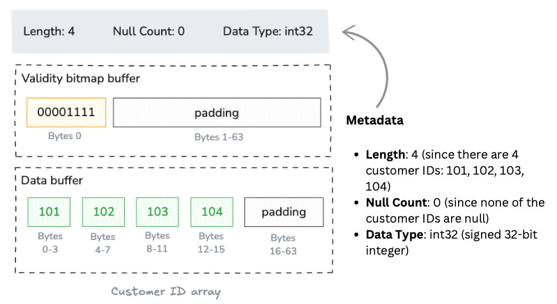
The Customer ID array results in a self-contained unit consisting of metadata (length and null count) and two buffers: a “validity bitmap buffer” and a “data value buffer”.

Let’s unpack the two buffers.
Validity bitmap buffer
Any value in an array may be semantically null, whether primitive or nested type.
All array types, except union types, use a dedicated memory buffer to encode the nullness or non-nullness of each value slot. We call this buffer validity (or “null”) bitmap. It is binary-valued, and contains a 1 whenever the corresponding slot in the array contains a valid, non-null value.
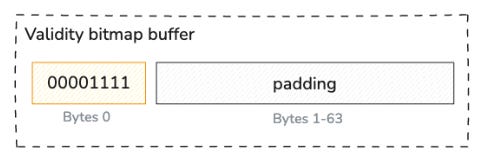
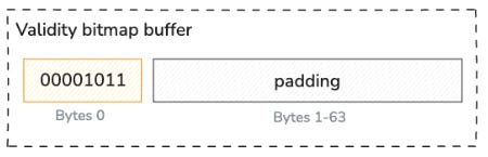
For our Customer ID column, all values are valid. At an abstract level, this would be a bitmap with all bits set to 1.
1111However, this is a slightly over-simplified version.
Because Arrow allocates memory in byte-size units, there are three trailing bits at the end (assumed to be zero), giving us the bitmap 11110000, represented in big endian format (the most-significant bit is written first, i.e., to the lowest-valued memory address)
Then, Arrow's byte ordering is little-endian by default. This means it is written in right-to-left order, giving us 00001111. Finally, Arrow adds padding (with 0s) to the remaining 63 bytes to align the buffer to a 64-byte boundary, optimizing for CPU cache lines.
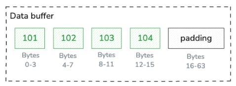
Data buffer
Finally comes the data buffer storing the actual integer values. Each value occupies exactly 4 bytes (32 bits) since we're storing 32-bit signed integers, with each containing a raw binary representation.
The data buffer, like the validity bitmap, is padded to a length of 64 bytes to preserve natural alignment.
Here’s the diagram showing the physical layout:
Each buffer in Arrow is stored as one continuous block in memory. However, when an array uses multiple buffers, these buffers don't have to be next to each other in memory. The metadata (like length, null count, and data type) is kept separate from the actual data buffers.
Storing fixed-size primitive arrays (with a null value)
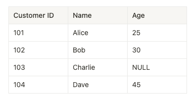
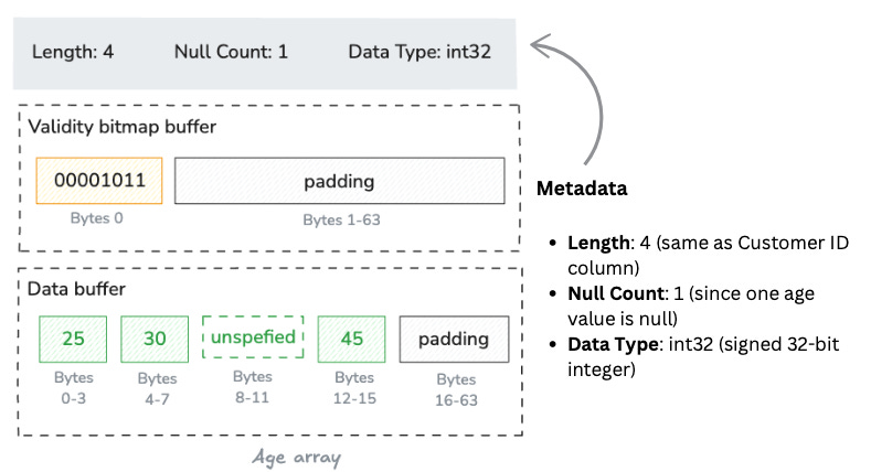
Next, if we ask Arrow to lay out the Age column for us, that would result in Arrow creating another primitive array of int32s. The difference this time is that our Age column contains a null value in one of its slots: the customer with ID 103 has a missing age value. So the validity bitmap would be 00001101.
The data buffer would still be allocated for all four integer values, but the bytes for the third position (customer 103) would be unspecified since it's null. This means the space is allocated for the value but those bytes are not filled.
Validity bitmap buffer
Unlike the Customer ID example where all values were valid (1111), the Age column has one null value at position 2 (zero-indexed). So the validity bitmap would be:
1101After expanding to byte-size and applying byte-ordering rules, we get:
Storing variable-size binary values
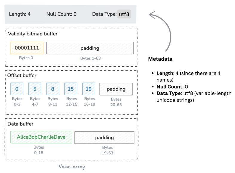
String arrays in Arrow have a more complex structure than fixed-size primitive arrays because strings can have variable lengths. Let's see how Arrow would represent the Name column from our data set.
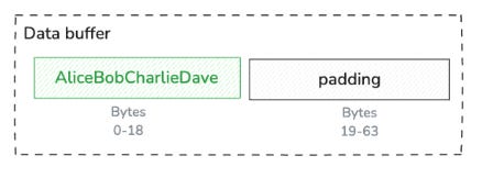
Arrow will represent our Name column, [Alice, Bob, Charlie, Dave], in a variable-size binary layout. While fixed-size primitive arrays have a single values buffer, variable-size binary arrays have both an offsets buffer and a data buffer. The additional buffer, the offsets buffer, stores the byte offsets that indicate where each string begins and ends in the data buffer.
Using the same schematic notation as before, this is the structure of the object. It has the same metadata as before but as shown below, there are now three buffers:
Offsets buffer
This is the key difference from primitive arrays. The offsets buffer contains (length + 1) 32-bit integers that represent the starting positions of each string in the data buffer, plus one final offset that marks the end of the last string.
For our example:
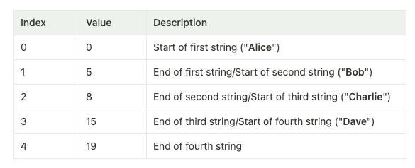
The offsets buffer with padding would be:
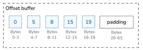
The data buffer contains all the string values concatenated together in one contiguous section of memory.
Putting it all together - Making up the Arrow Table
Now that we've examined how Arrow stores primitive arrays (Customer ID and Age) and string arrays (Name), let's see how these individual arrays come together to form a complete Arrow table.
An Arrow table is composed of three elements:
Schema: Defines the structure of the table, including field names and data types
Record Batches: Horizontal slices of the table containing the actual data
Columns: The individual arrays we just examined
For our customer data example, the table consists of the three arrays laid out in a columnar format
Column 1 (Customer ID): A primitive array with validity buffer and data buffer
Column 2 (Name): A string array with validity buffer, offsets buffer, and data buffer
Column 3 (Age): A primitive array with validity buffer and data buffer
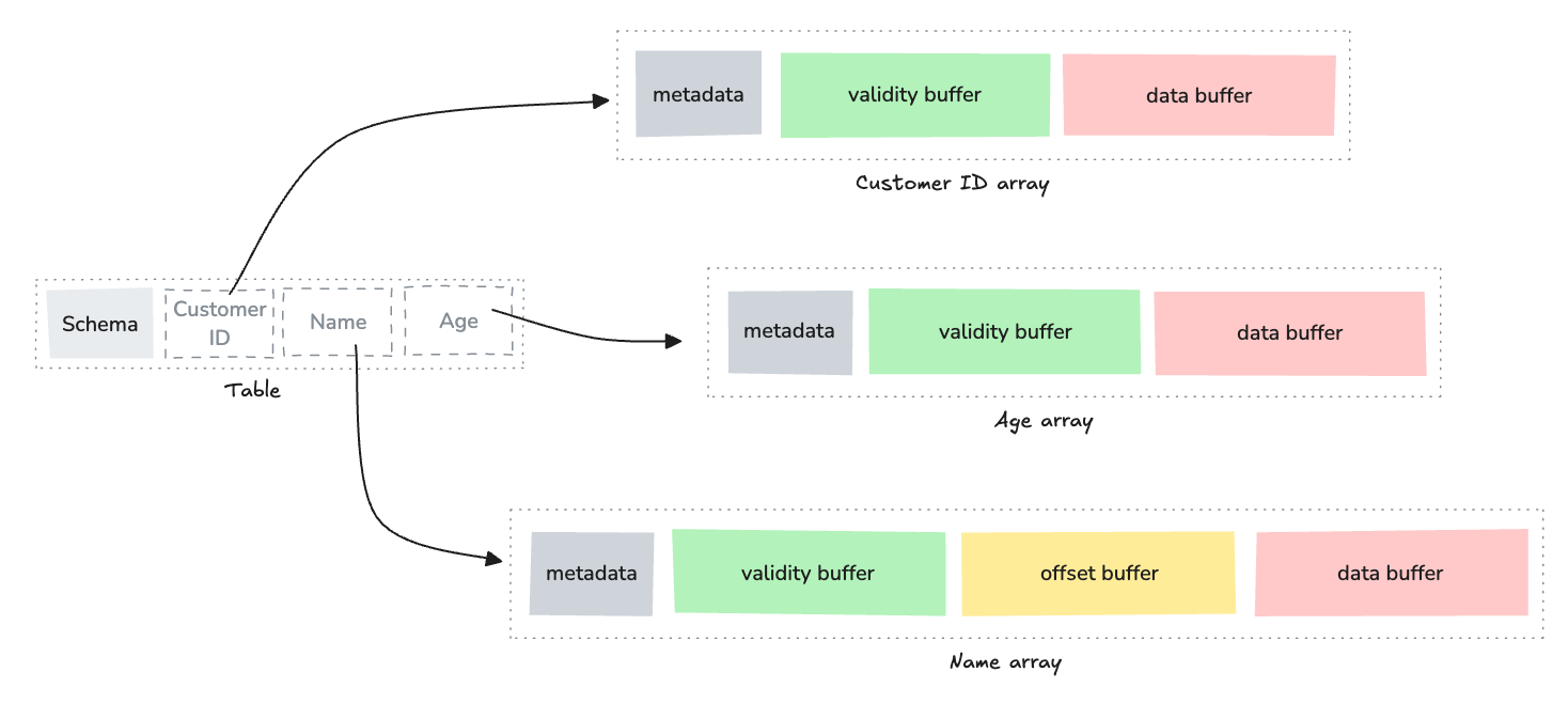
This is a dramatically simplified version of the Arrow table memory layout. I will discuss more on that in a future post. The key point is that each table column is stored as a contiguous array in memory, rather than storing each row together. This is the essence of columnar storage.
Arrow is actually creating the exact memory layout we've discussed, with each array having its own buffer(s) and metadata, all organized in a columnar format according to the Arrow specification.
This memory-efficient representation makes Arrow ideal for data processing systems that need to handle large datasets and share them across different programming languages and tools.
Wrapping up
In conclusion, Apache Arrow's columnar memory format isn't just for efficient in-memory analytics—it's designed as a universal interchange format enabling seamless data sharing across different contexts. For sharing with other processes, Arrow leverages zero-copy Inter-Process Communication (IPC), allowing multiple processes to access the same memory buffers without duplicating data, significantly improving performance for data-intensive applications.
To persist data on disk, Arrow offers the Arrow File Format (stored as .arrow files) and the Arrow IPC Stream Format. These formats maintain the columnar structure and can be memory-mapped directly into applications, eliminating costly serialization/deserialization steps common in traditional file formats. The Feather format, built on Arrow, provides a lightweight solution specifically for data frame storage.
For network transmission, Arrow integrates with protocols like gRPC and Flight, a specialized protocol built on top of Arrow that optimizes for high-throughput data transfer between services. This allows distributed systems to exchange data efficiently while preserving the columnar structure, enabling remote processes to work with the data as if it were local.
Each of these sharing mechanisms maintains Arrow's core principle: avoiding unnecessary data conversion while preserving the performance benefits of columnar storage. In the next post, I'll explore these data sharing capabilities in greater detail, demonstrating how Arrow enables a new level of interoperability in data processing ecosystems.